👨🏫 Mathematics
Demystifying Probability Distributions ( 2 / 3 )
(2/3) More on discrete random variables, continuous RVs, the CDF
In the previous part, we educated ourselves around discrete random variables and the probability mass function. As a quick recap, probability mass functions are probability distributions for discrete random variables. In the end of the previous post, we also had a quick glance of the Bernoulli Distribution but this time we would have a more thorough and formal treatment for it. Meanwhile, we also introduce other important probability distributions for discrete random variables.
In case you missed the 1st part,
Bernoulli Distribution

This is a discrete probability distribution, meaning it can be used to express probabilities for random variables that have finite or countable outcomes. This implies that discrete probability distributions are only for discrete random variables ( recall the definition of a discrete random variable ).
Bernoulli Distribution is best conceptualized by the simple coin toss experiment with a biased coin. The probability that the coin shows up a heads is p which implies that the probability of getting a tails is 1 — p. If a random variable X takes two values 0 and 1 ( hence, discrete ), with probability of having value = 1 with probability p, we can say that X follows a Bernoulli Distribution,

The Bernoulli Distribution is named after Swiss mathematician Jacob Bernoulli.
Where p is the parameter of the Bernoulli distribution, as described above. The probability mass function of the Bernoulli distribution is given by,

Or equivalently,

Note: As we are allowing 0 ≤ p ≤ 1, we cannot say that the support of X is { 0 , 1 }. You must recall the definition of support from the previous part.
We could simply the notation for the PMF by expressing it as function f with parameter p,

Recall the ice-cream shop experiment we took in the previous blog. We considered a random variable which represented the two choices made by a customer viz. a chocolate or a vanilla ice-cream. Applications of the Bernoulli distribution might seem simple and obvious, but they can help us understand other discrete probability distributions which are the generalizations of the Bernoulli distribution.
Binomial Distribution
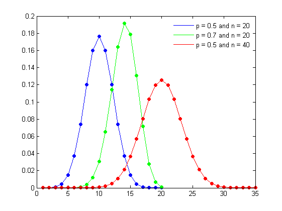
Suppose you’re performing 10 coin tosses, with a biased coin. The biased coin can show a tails with a probability p, and indeed a heads with probability 1-p. Consider a discrete random variable Y which indicates the number of heads/tails we’ll get in the experiment of performing 10 coin tosses. If we want to determine the probability of getting exactly 6 tails out of the 10 coin tosses, I would search for p( Y = 6 ). The discrete random variable Y can take values { 0, 1, …, 10 } each with some probability. Such a discrete random variable is said to be distributed according to a Binomial Distribution,

Where n is the number of trails. or in our case, the number of coin-tosses performed. p is the probability of the outcome whose count is specified by Y. In our case, we perform 10 coin tosses, hence n = 10. Y specifies the number of times we’ll get a tails, so p represents the probability of a biased coin showing a tails ( we established this earlier ). The PMF of such a random variable is given by,


The PMF of the binomial distribution might look similar to the expression of binomial expansion, but they are totally different!
If we wish to find the probability of getting 6 tails, considering p = 0.6, then we need to determine f( 6 | 10 , 0.6 ),

So there’s only 25.08 % chance of getting 6 ( which equals x ) tails out of 10 ( n ) coin-tosses, where the chances of each coin showing a tails is 60 % ( p ) .
Here comes the interesting part. Notice that when n = 1 for the Binomial Distribution, we get the PMF of the Bernoulli Distribution. Binomial Distribution consists of multiple experiments where each experiment can have two outcomes, just as we considered n coin tosses in the beginning.
To know more on how the PMF is derived, here’s a great video by 3Blue1Brown.
Poisson Distribution
Imagine yourself in a pizza shop. You have been assigned the task, by the manager, to model the number of calls received throughout the day. To help you with the task, the manager has provided you some data regarding the number of calls received per day.
On holidays, the number of orders ( or the calls received at the shop ) could go upto 100, whereas during the week days, the number of calls is quite less, around 34. You compute the average of the number of calls each day, which comes out to be 51 calls per day. But how would this accomplish the task of modelling the number of calls received each day at the pizza shop?
Consider a discrete random variable X, which can take values 0, 1, 2, 3, … and it represents the number of orders ( calls ) received in a single day. As our average rate of calls comes out to be 51 calls a day, we expect that the number of calls received each day would revolve around this number only. Also, each call is independent. No two calls could have an influence on each other.
In order to satisfy these ideas, we can say that X is distributed according to a Poisson Distribution,

The Poisson Distribution is named after French mathematician Siméon Denis Poisson.
Observe the parameter λ, which is the rate of the event taken into consideration. The PMF is given by,


In the above PMF, x represents the number of times the event occurs, hence it is non-negative. Considering our example, λ could be the average rate at which the pizza shop receives calls in a day. So, λ equals 51.
Let us calculate the probability of getting 50 calls per day ( observe, this value is closer to the average number of calls a day ),

Here’s a plot which shows the probability vs. number of calls received for an average rate of λ = 51,
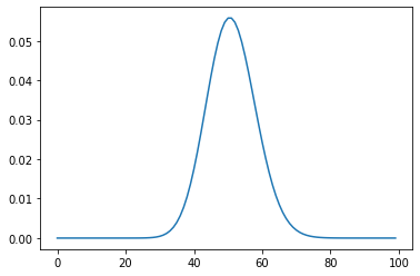
The maximum probability is observed at X = 50. For X = 5 and X = 100,


As you may observe the probabilities of getting 5 or 100 calls a day is very less.
All the above calculations, were made using Python. See the code here.
This might not be noticeable at the first glance, but the Binomial Distribution approaches a Poisson Distribution as n→∞. The derivation requires good knowledge of solving limits, and hence we would skip it here. Here’s a good read on it,
Continuous Random Variables
Continuous random variables can attain continuous ( or infinite ) values within some interval. If we consider a continuous random variable Y which take values in the interval [ 0 , 1 ], it is obvious that Y can take infinite real values. In a simple coin toss experiment, if the probability of getting a heads is p then the probability of getting a tails is 1-p, which is evident as the *sum of probabilities of all possible outcomes must equal 1. As Y can take infinite values, we can have an infinite number of outcomes, so how do we assign probabilities to each one of these?
As the number of outcomes increase, the probability of each outcome would decrease. Taking the number of outcomes to infinity, the probability of each outcome squeezes to zero. Hence, while discussing continuous random variables, we don’t bring in the probabilities of individual outcomes. Like, we would never discuss the probability of Y attaining a value of 0.5,

Instead of individual values, we would talk about the probability of Y attaining some value in a given interval, like,

In a gist, we’re asking the question, ‘What is probability of Y attaining a value in the interval [ 0.1 , 0.2 ]?’
Cumulative Distribution Function
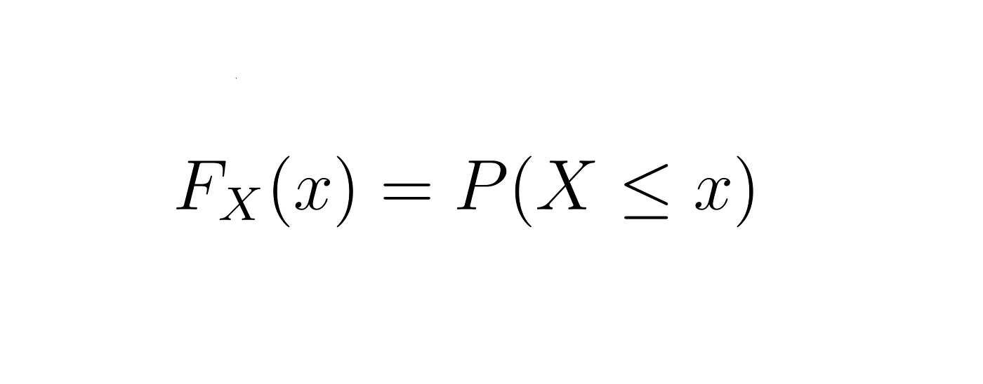
In our discussion above, we considered a continuous random variable Y which can take values in the interval [ 0 , 1 ]. What if we need to determine the probability of Y attaining values which are smaller or equal to some particular value? For time being, we wish to determine the probability of Y attaining a value smaller than or equal to 0.3. The cumulative distribution function ( CDF ) of the continuous random variable could be used in such a case. It is defined as,

Also, we consider that y belongs to the interval [ 0 , 1 ]. The CDF possess some interesting properties, like,
- In this series, we’ll study CDFs for continuous random variables only, but remember, CDFs can be defined for discrete random variables as well.
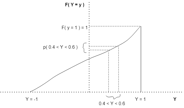
- The CDF is a monotonically increasing function. Meaning, as y increases, the value of F( y ) also increases.

- As we discussed in the previous section, the probability of Y attaining values in the interval [ 0.1 , 0.2 ], can now be determined using the CDF of Y.


As the probability at individual points ( like P( y = 0.1 ) or P( y = 0.2 ) ) is zero, P( 0.1 ≤ y ≤ 0.2 ) = P( 0.1 < y < 0.2 ) = P( 0.1 ≤ y < 0.2 ) = P( 0.1 < y ≤ 0.2 )
- For the CDF of a continuous random variable X, as x approaches negative infinity, the value of the CDF function also approaches zero. Similarly, as x approaches positive infinity, the value of the CDF function also approaches one,

Considering the random variable Y, from our previous discussions,

This is because, by definition y belongs to the interval [ 0 , 1 ]. Hence instead of approaching positive and negative infinity, y can only approach 1 and 0 respectively. And, that’s all about the CDF.
The CDF will help us understand the PDF, or the probability density function, which we’ll cover in the next part. Also, we’ll discuss more on some continuous random variables, just as we did for discrete random variables.
See You In The Next Part!
Hope you loved this story. Do share your comments, suggestions and improvements in the comments below, or send me a message on equipintelligence@gmail.com.
Thanks for reading, and have a nice day ahead!
